AI methods from the field of machine learning are used here that allow the user to accurately model complex relationships without requiring precise knowledge of the algorithms in the background. The software is therefore used by a wide range of users. They include less experienced users, who appreciate parameter-free, automated model creation, as well as experts, who are given all the freedom they need thanks to the extensive configuration options available.
A typical application of ASCMO-STATIC is the modeling of the fuel consumption and pollutant emissions of complex internal combustion engines as a function of engine speed, load, and all the engine control variables. Accurate predictions can be made, and manual and automatic optimizations can be implemented based on these models. This makes it possible to achieve the best compromise between pollutant emissions and fuel consumption as well as other boundary conditions during engine operation.
Benefits
- Easy to use with no specialized knowledge required
- Powerful AI methods from the field of machine learning
- Interactive graphical representation of multidimensional dependencies
- Ability to share models and data using standardized formats
- Reduction of model complexity for time-critical applications, such as deployment in ECUs
- Powerful MATLAB® and COM interfaces for integrating customer-specific functions and tools as well as for linking to test-bench automations
Features and Functions
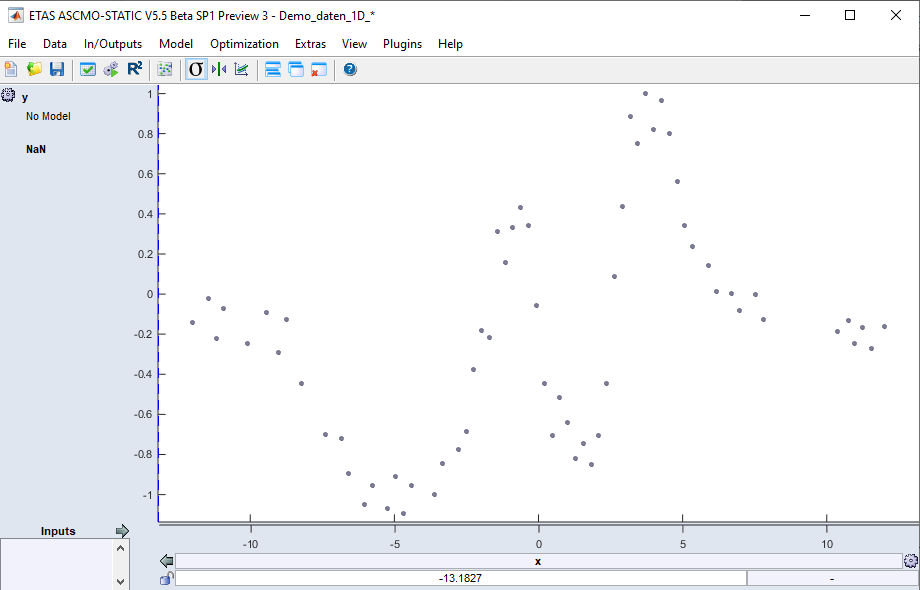
Since data-based modeling is used in ASCMO-STATIC, this data must typically be obtained through measurements on a real system. An essential element for this is the design of experiments (DoE), which enables a maximum model accuracy to be achieved with a minimum of effort spent on measuring.
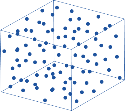
The DoE experimental design module (ExpeDes) makes it easy to plan the underlying measurements. Using design of experiments methods, the positions of measuring points where measurements are obtained are proposed methodically and in a space-filling way. The variation range of the parameters to be adjusted can be limited graphically or numerically in up to four dimensions in each case. Using a formula editor, this is possible in any number of dimensions. Thanks to an intelligent division of the experimental design into blocks, it is possible to adjust the time and effort required for measuring so that it is commensurate with the degree of accuracy desired. In addition, the sort order of the measuring points as well as a compression of the points in certain regions of the experimental space can be set. Requirements concerning test bench automation (e.g. sorting and arrangement of operating points) are also taken into account in a highly practical way. Graphical representations of the points in all dimensions facilitate straightforward validation and evaluation of the DoE plan.
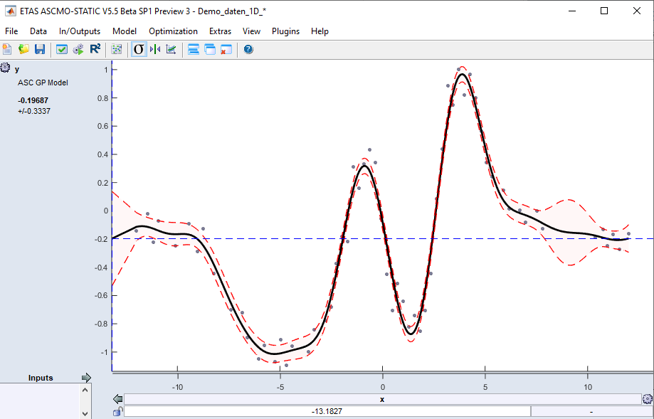
The main function of modeling in ASCMO-STATIC is to enable accurate, straightforward, and robust prediction of the system behavior. The tool makes it easier for less experienced users to use the advanced modeling methods required for this, but at the same time it gives experts the freedom to adjust the model parameters with a high degree of flexibility. In ASCMO-STATIC, the modeling is based on Gaussian process models. This consists of a statistical learning method using measurement data based on Gaussian processes that has already proven its worth many times. With this, the specific mathematical function that best represents the real system behavior is determined automatically.
Creating such a model is very easy. After selecting the relevant inputs (influencing variables) and outputs (target values) of the system, the user can immediately initiate training the model without further parameterization.
The time required for model training depends on the number of measuring points and inputs and typically takes around a few seconds up to a few minutes. Experienced users can activate expert mode, which gives them access to all the model options and parameters and thus allows them to make specific adjustments when needed that have an influence on the model training. The model quality is indicated by easy-to-understand charts and key figures.
Further advantages of Gaussian process models:
- Measurement noise is taken into account, so overfitting can be avoided
- Robustness against measurement outliers
- Locally resolved model variance gives the user a measure of the reliability of the model prediction
In addition to the standard modeling method, the tool also provides other algorithms for special tasks. This includes models for classification and reducing complexity. All models can also be exported in different formats and used freely outside ASCMO as a so-called plant model. Common examples of the possible formats are Simulink, C code, and FMU/FMI.
A special format is available for creating an export for use on the Bosch AMU (Advanced Modeling Unit hardware accelerator). The AMU is a special module on the Bosch MDG1 ECU and is used for evaluating the ASCMO model stored on it in volume-production vehicles.
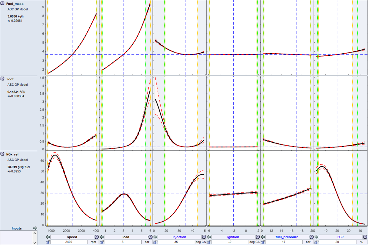
One of the standard views for visualizing the models is the so-called intersection plot. These interactive intersection plots allow multidimensional dependencies to be displayed in a straightforward way. The x‑axis displays the inputs to the system, and the y‑axis displays the outputs.
In each sub-graph, the black line (model prediction) shows the influence of an input (x‑axis) on the corresponding output (y‑axis). In other words, if the input is varied, the real system would influence the output in the way shown by the black line – as long as all the other inputs are not adjusted. As soon as another input is adjusted, this dependency can change. This shows how the interactions of the inputs have an effect on the output. A red dashed line is also displayed above and below the black line that indicates the reliability of the model prediction. The closer it runs alongside the black line, the more certain the model is that the prediction can be calculated reliably.
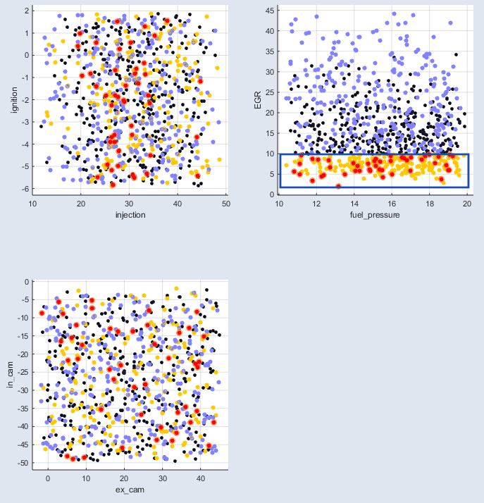
Besides this main view in ASCMO-STATIC, there are also various other options available for visualizing the dependencies and influences. This also includes, for instance, the ability to display calibration maps or the scatter plot, which can present the data as a point cloud in any number of different combinations.
The user therefore has a whole range of options available for analyzing and visualizing the behavior of the modeled system. It provides a straightforward way of carrying out validation tasks and establishing an understanding of the system without having to perform complex and time-consuming measurements on the real system.
To optimize the input variables for controlling e.g. an engine, it is possible to define various criteria, such as minimization/maximization, upper/lower limit values, and target values for the output variables. During optimization, these criteria can either be weighted or the complete trade-off curve (Pareto curve) can be calculated. The user can then select the appropriate compromise from the trade-off curve. For engine applications, a global optimization can be carried out over the entire operating range. The user then receives an optimal calibration of the characteristic maps of all input variables in a very short time. The characteristic maps can also be adjusted manually or locked. The user always sees the effects of the changes on the output values immediately. This is true for the individual value at the current operating point as well as for the cumulative value with respect to the complete driving cycle.
The results obtained from the optimization can be exported in various formats. When it comes to engine management calibration, the usual formats are DCM or CDFX. The Excel formats XLS and XLSX as well as the CSV format are also supported.
In ASCMO-STATIC, the models can be used as a virtual measuring instrument for artificially generating large amounts of measurement data. For this purpose, the user can define any grid sizes for the input variables in terms of step size, number of steps, and free break points directly in the tool or by importing Excel lists. For all the desired parameter combinations of input variables, the model will then calculate the corresponding output variables. Just like real measurements (e.g. from the engine test bench), this artificial measurement data can be used, analyzed graphically, and exported as a CSV file for further processing in Excel.
Compatibility
ASCMO-STATIC is open and flexible. The tool supports all relevant data formats that are used, for example, on the test bench and in calibration. ASCMO-STATIC can export the created models in various formats for use in other environments. Using the MATLAB® interface, the user can easily integrate customer-specific functions and models, automate operations with scripting, or incorporate a test bench automation. It is also possible to connect a test bench automation via the COM interface.